Once a referential range R is specified, the extensions of the various sorts of non-logical vocabulary can be specified in ways that extend those used in truth-functional logic. Individual terms are merely assigned reference values from R in the way sentences were assigned truth values. The extensions of predicates and functors are functions and, as we have already seen, these can be indicated by tables analogous to truth tables. Below is an example of an extensional interpretation of the following non-logical vocabulary:
| sentences: | A, B |
| individual terms: | a, b, c, d, e |
| predicates: | F (1-place), G (1-place), R (2-place) |
| functors: | f (2-place) |
We choose (arbitrarily) a referential range with five values whose IDs run from 0 to 4 and assign (again arbitrarily) extensions of the appropriate sorts to the items of non-logical vocabulary.
| R: 0, 1, 2, 3, 4 |
|
|
|
|
|
|
The truth-table row giving the values of A and B is dwarfed by the other information in the structure, but the whole of the structure has the same significance for our present analysis of logical form as did the left side of a single row of a truth table in truth-functional logic.
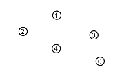
Since we build in no assumptions about the size of the range R, we can consider structures that are quite small, and it is possible to represent small structures in pictorial diagrams. As in Figure 6.4.2-1, let us depict a range by a rectangle, with the values of the range shown as circles that enclose numbers, which will serve as the IDs of the reference values in the range.

Fig. 6.4.2-1. A range of reference values labeled by their IDs.
The extension of a simple term will be one of these reference values, and we can show this by writing the term next to that value. Figure 6.4.2-2 shows the extensions assigned above to the terms a, b, c, d, and e. The terms b and e are written next to the same value because both were assigned that value as their extension.
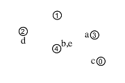
Fig. 6.4.2-2. A range with the extensions of five terms shown; two have the same extension.
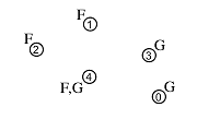
The extension of a one-place predicate is a function that yields a truth value as output when it is applied to a reference value as input. We will say that it is true or false of a reference value depending on its output for that value as input. We can represent this sort of extension by writing the predicate next to the values it is true of; we will then know that it is false of any other reference values. Figure 6.4.2-3A does this for the predicates F and G, again using the extensions originally given in tables.
A |
B |
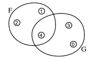
Fig. 6.4.2-3. A range with the extensions of two one-place predicates indicated by labeling values (A) and enclosing sets of values (B).
This can make the diagram rather cluttered, but we can clean things up a little by drawing a line around all the values a predicate is true of and labeling the line rather than the values. This is done in Figure 6.4.2-3B. The second sort of diagram corresponds fairly directly to what was the original concept of an extension—the class of things a predicate is true of—and we can say that the values a predicate is true of are in its extension.
Predicates with more than one place are not true or false of single values but of pairs, triples, or longer series of values. For example, λxy (x is the father of y) is true not of James Mill or of John Stuart Mill (his son) taken individually but instead of the two taken together and in that order. Such an ordered pair of values can be represented in our diagrams by an arrow from its first to its second member. (We could represent longer series of values by adding legs between the head and tail of the arrow.) The extension of a 2-place predicate can be thought of as the collection of pairs it is true of. Similarly, the extension of a 3-place predicate will be a collection of triples, and the extension of a predicate with some number n of places will be a collection of n-tuples (i.e., of series with length n).
There are a number of ways a collection of n-tuples can be depicted. We might draw the arrows that represent its members and label each one as we initially labeled the values in the extension of a one-place predicate. This would make for some more clutter, but it would be hard to avoid that by drawing a line around a group of arrows. We might write the predicate once and draw a line from it to each of the arrows in its extension, or we might draw different styles of arrows for different predicates, labeling the style of arrows in a legend like that of a road map. Each of these three approaches to labeling the extensions of many-place predicates has its value but we will most often use legends. Figure 6.4.2-4 shows this latter style of diagram for the extension that was assigned to the 2-place predicate R. Notice that the predicate is true of the values 1 and 2 taken in either direction and that it is also true of each of 3 and 4 paired with itself (and look back to see how that information appeared in the table).
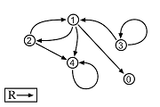
Fig. 6.4.2-4. A range with the extension of a 2-place predicate indicated.
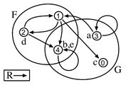
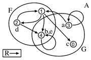
Figure 6.4.2-5A combines the extensions of the three predicates. As was noted in 6.1.4, unanalyzed sentences can be thought of as zero-place predicates. That means that they do not express properties that may or may not be true of objects or relations that may or may not hold between objects. Instead sentence express state of affairs that are simply true or false. One way to indicate that in a diagram is to simply include a true sentence within the rectangle, understanding any unanalyzed sentence that does not appear there to be assigned the value F. That addition to the diagram is shown in Figure 6.4.2-5B.
A |
B |
Fig. 6.4.2-5. A range with the extensions of predicates (A) and predicates together with the indication that a sentence is true (B).
All that is left are the extensions of functors. We could use arrows here, too, because a reference function establishes a relation between its input and output values. For example, the squaring function relates 1 to itself, 2 to 4, 3 to 9, and so on. However, this would make for a lot of arrows. A one-place function relates each value to some other value (perhaps the nil value), so each value would be at the tail of an arrow; and things get much worse with functions of two or more places. We can get a somewhat more compact notation by adapting the way we indicate the extensions of individual terms. Next to each output value of a functor, we can write the functor with its places filled by IDs of the input values for which it yields that output (for example, writing f01 next to the value 2 to say that 2 is the output of f for inputs 0 and 1). Since the extension of a functor may yield the same output for different input values, we may need to write the functor next to an ID several times, each time filling its places with the IDs of different input values. This is manageable for 1-place functors because, for each such functor, we will need only as many labels as there are possible input values—i.e., one for each member of the range. But for a function with two places, the number of labels is the square of the number of reference values and this number mounts rapidly. In the example we are considering, we would need to write the 2-place functor f 25 times to indicate all 25 entries of the table shown earlier. Adding to these only the individual terms leads to the rather cluttered diagram shown in Figure 6.4.2-6.
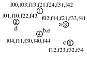
Fig. 6.4.2-6. A range showing the extensions of a 2-place functor and several individual terms.
Most of the structures we consider will be quite small, and this approach will be more feasible with them. Still, it is always possible to supplement a diagram with one or more tables, and that is the easiest approach for the example we have been considering. The full interpretation is given in this way in Figure 6.4.2-7.

|
|
Fig. 6.4.2-7. A structure for a variety of non-logical vocabulary.
Now let us do something with this structure. Interpretations are assigned in order to settle the truth values of sentences formed using the vocabulary that is interpreted. This is analogous to calculating a truth value of a truth-functional compound given an assignment of truth values to its ultimate components. Below is the calculation of the truth value given to a sentence by the structure we have been considering. It is followed by an explanation of the initial steps in the process; this explanation refers to the way the interpretation is presented in the diagram and table in Figure 6.4.2-7.
|
|||||||||||||||||||||||||||||||||||||||||||||||||||
| Ga: | a has 3 as its value and this value is in the area representing the extension of G, so Ga gets T | ||||||||||||||||||||||||||||||||||||||||||||||||||
| Rde: | d and e have 2 and 4 as their extensions and the arrow for this pair is in the extension assigned to R, so Rde gets T | ||||||||||||||||||||||||||||||||||||||||||||||||||
| F(fab): | f yields the value 0 when given the extensions of a and b (the values 3 and 4) as input (as can be seen from the end of the next-to-last row of the table for F), and 0 is not in the area marked as the extension of F; thus fab gets 0 and F(fab) gets F | ||||||||||||||||||||||||||||||||||||||||||||||||||
| B: | B gets the value F since, unlike A, it does not appear within the rectangle | ||||||||||||||||||||||||||||||||||||||||||||||||||
| b = e: | b and e both have 4 as their extension, so b = e gets T |
The extensions of complete unanalyzed expressions have been written under these expressions, and the values of compounds are written under signs for the operations that form them. As in truth-functional logic, the order of calculation is determined by parentheses. Notice that capital letters always have truth values under them and lower case letters always have reference values under them.